README.md

genoxide for Python

The algorithms of genoxide, a Rust library, with fitness functions in Python and numpy:

• genetic algorithms, local search and the Nelder-Mead simplex method
• L-BFGS-B for smooth functions with a gradient, yours, finite differences or the test problems' own
• first-order gradient methods for up to millions of parameters: gradient descent, momentum, Nesterov, Adam and AdamW
• MMA and GCMMA, the method of moving asymptotes, for millions of variables with few constraints, from gradients
• Bayesian optimization for expensive functions, in batches evaluated in parallel, with constraints and on integer genes, with Gaussian processes (gx.model.gp) you can also fit on their own
• continuation: a gradient method through stages of one problem, its state kept between them
• differential evolution, evolution strategies, CMA-ES and particle swarm optimization
• NEAT, OpenAI's evolution strategy, neural networks and pole-balancing tasks, for neuroevolution
• genetic programming: formulas and Boolean functions as trees, with symbolic regression and Koza's problems evaluated in Rust
• the island model, and checkpoints to resume a long run
• NSGA-II, NSGA-III, SPEA2, MOEA/D and SMS-EMOA for several objectives

The API reference: tachsin.github.io/genoxide/api/python

import numpy as np
import genoxide as gx

# OneMax: the genome with the most ones
ga = gx.Ga(
    gx.Binary(100),
    population_size=100,
    select=gx.Tournament(3),
    crossover=gx.UniformCrossover(),
    mutation=gx.BitFlip(rate=0.01),
    seed=42,
)
result = ga.run(lambda bits: bits.sum(), target=100, generations=1_000)
print(result.best_fitness, result.generations)

# Rastrigin with CMA-ES and IPOP restarts, a generation per call
def rastrigin(x):  # x: a genome per row
    return 10 * x.shape[1] + np.sum(x**2 - 10 * np.cos(2 * np.pi * x), axis=1)

cmaes = gx.Cmaes(gx.Real((-5.12, 5.12), length=10), restarts="ipop", objective="minimize", seed=1)
result = cmaes.run(rastrigin, batch=True, target=1e-8, evaluations=500_000)
print(result.best_genome, result.best_fitness)

More in examples/, each the same program in Python and Rust (python examples/<name>/main.py in the repository), on the docs site, and played back with charts made for each problem on tachsin.gr:

• OneMax, LeadingOnes, the deceptive trap, the royal roads, an NK landscape, a knapsack with a constraint, and N-Queens
• the travelling salesman (TSPLIB berlin52) and job shop scheduling (ft06)
• Rastrigin with CMA-ES and L-SHADE, and the pressure vessel and welded beam designs with constraints
• the gear train design, an integer problem
• CMA-ES, SHADE and PSO on twelve test functions, and Himmelblau's four minima by restarts of a local search
• ZDT1 with NSGA-II, and DTLZ2 with NSGA-III
• the constrained BNH with NSGA-II, and Kursawe's disconnected front with SPEA2 and NSGA-II
• XOR neuroevolution with CMA-ES, and the two spirals with OpenAI's evolution strategy

Install

pip install genoxide

Wheels for CPython 3.10 or later, and for free-threaded CPython 3.14 (3.14t), with numpy:

• Linux: x86_64 and aarch64, glibc and musl
• macOS: Apple silicon and Intel
• Windows: x64

To build from the repository, with Rust and maturin:

cd python
pip install maturin
maturin develop --release

Fitness functions

A fitness function takes a genome as a numpy array:

Genome	Array
Binary(length)	bool
Integer(bounds, length)	int64
Real(bounds, length)	float64
Permutation(length)	int64, an ordering of 0 .. length - 1
AdaptiveReal(real, initial_step)	float64, the genes of real, without the step size that evolves with them
gx.gp.Gp(primitives)	not an array: a gx.gp.Tree, see Genetic programming

bounds is one pair (low, high) for every gene, with length, or a list of pairs, one per gene.

It returns one of these:

• a number
• None or NaN, for a solution that can't be scored
• (score, constraint_violation): a positive violation marks an infeasible solution. Infeasible solutions rank below feasible ones, and among themselves by violation (Deb's rules).

The fitness function must be deterministic: genoxide doesn't evaluate again a child identical to one of its parents.

With batch=True, the function takes a whole generation as a 2-D array, a genome per row. It returns:

• an array of scores, or a tuple of scores and constraint violations (arrays or (n, 1) columns)
• for several objectives, a 2-D array or a list with a row of objective values per genome, or a tuple of one array per objective (return f1, f2)

It's one call per generation, and none for a generation whose children are all copies of their parents. Vectorized numpy, a GPU or a remote service pays its cost per call once per generation, not once per genome. The next call of as many genomes gets the same matrix back, written again, if the function kept no reference to it: a large matrix is allocated once per run. A function that keeps its matrix, or a view of it, gets a new one next time, and what it kept never changes.

With parallel=True, genoxide calls a non-batch function from several threads at once. It pays off when the function releases the GIL (numpy on large arrays, waiting for I/O), or on free-threaded Python (3.14t).

An exception in the fitness function stops the run, and run raises it. So does Ctrl+C: with parallel=True, once the calls under way return, without starting the others.

Choosing an algorithm

Problem	Genome	Algorithms, the first preferred
Yes / no choices (subsets)	Binary	Ga with UniformCrossover() or PointCrossover(points), and BitFlip
An order (tours, sequencing)	Permutation	LocalSearch, which often beats a GA on permutations; Ga with OrderCrossover() (sequences) or EdgeRecombinationCrossover() (tours)
Reals in ranges	Real	Cmaes; De; Es; Ga with SimulatedBinaryCrossover(eta) and PolynomialMutation(eta); Lbfgsb for a local minimum of a smooth function, any number of genes; NelderMead for a local minimum in a few dimensions
An expensive function of a few reals or integers (tens to a few hundred evaluations)	Real, Integer	Bo, Bayesian optimization, up to about 10 to 20 genes
A smooth function of many reals, with its gradient	Real	FirstOrder (Adam, momentum, Nesterov), up to millions of genes
Smooth, with gradients: very many reals (up to millions), few inequality constraints	Real	Mma; method="gcmma" to converge from any start
A neural network's weights	Real, from network.representation(bounds)	Cmaes up to a few hundred weights; OpenEs for thousands and more
A neural network's structure and weights	gx.neat.Network, NEAT's own	Neat
A formula or a Boolean function (genetic programming)	gx.gp.Gp, trees	Ga with gx.gp.SubtreeCrossover() and gx.gp.SubtreeMutation(), or Islands of them; Nsga2 for accuracy against size
Several objectives	any	Nsga2 for 2 or 3 objectives; Nsga3 or Moead for more

• Cmaes is the strongest general choice for continuous problems with up to a few hundred genes, especially when the genes interact. Its defaults need no tuning. For multimodal functions, add restarts="ipop" or "bipop". restarts="stop" ends a run once it converges, with the stop reason "converged": for smooth problems without constraints, as on flat, quantized or constrained fitness a run can still improve after it converges. For thousands of genes or separable problems, covariance="diagonal" (sep-CMA-ES): O(n) per sample, no correlations between genes.
• De often needs far fewer evaluations than a GA on continuous problems.
• Pso with ring=1 explores longer than the default global topology, for multimodal functions.
• Es, an evolution strategy whose step sizes evolve with its solutions, suits smooth problems that need precise answers. A Ga on an AdaptiveReal genome with SelfAdaptiveMutation() is one too.
• OpenEs, OpenAI's evolution strategy, follows a gradient estimated from mirrored samples, at a cost per sample linear in the genes: for thousands of genes and more, such as a network's weights.
• NelderMead is a local method without derivatives: it converges to the minimum of the basin it starts in, from initial_genome or a random point, and stops there (the stop reason "converged"). It suits up to about 10 genes, and functions that are non-smooth or noisy in their last digits. restarts=n starts again n times from random points, for multimodal functions; speculative=True evaluates the steps of an iteration in one round, for a slow function evaluated in parallel.
• Lbfgsb (L-BFGS-B) is the local method for smooth functions: with the gradient, it reaches the minimum in the bounds to many digits in far fewer evaluations than the others, from a few genes to millions. Give it with run(f, gradient=g) (or gradient=True and f returning (value, gradient)); without one, it uses forward differences, a point more per gene for each gradient; a problem of gx.problems gives its own, in Rust. It stops on its own once converged (the stop reason "converged"). It polishes what a global method found: initial_genome=result.best_genome.
• FirstOrder steps along the gradient of a smooth function by a step rule, without a line search: step="adam" (Kingma and Ba's, the default), "adamw" (with decoupled weight decay), "momentum", "nesterov" or "gradient". One gradient per generation, from run(..., gradient=...) as for Lbfgsb, from a problem of genoxide.problems in Rust, or by finite differences (n more evaluations per generation, up to 10,000 genes). Memory and work per step are linear in the genes, for up to millions of them. It stops with the stop reason "converged" when the gradient vanishes; a control lowers the learning rate over the run (a schedule), which Adam needs to settle on the minimum.
• Mma, Svanberg's method of moving asymptotes, uses the gradient of the score and of each inequality constraint g(x) <= 0: the gradient as for Lbfgsb (no finite differences), and with run(f, gradient=True, constraints=m), f returns (value, gradient, g, jacobian), g the constraints' values and jacobian an array of a row per constraint. An iteration is one evaluation and a few passes over the genes, with no matrix of them: for up to millions of genes and up to a few hundred constraints. It stops on its own once it has converged (the stop reason "converged"). method="gcmma" converges from any start, at the cost of more evaluations; constraint_cost must exceed the constraints' multipliers.
• Continuation runs FirstOrder, Lbfgsb or Mma through stages of one problem, a smooth version first and sharper ones after (a smoothing that shrinks, a p-norm's p that grows, a penalty raised): on_stage(index) sets the stage's parameters for the fitness function, and the method goes on from its point with its state (Adam's averages, MMA's asymptotes; keep="point" keeps only the point). A stage ends when the method converges or after generations; the run, after the last stage.
• Bo, Bayesian optimization, is for expensive functions, where each evaluation counts: a Gaussian process (gx.model.gp) models the function from every evaluation, and an acquisition function of its posterior chooses the next point, one per generation after an initial design of 2(n + 1) points. The log expected improvement by default; "ei", gx.ProbabilityOfImprovement(xi) and gx.UpperConfidenceBound(beta) (whose beta a control can change). output="log" models the logarithm of the values, for objectives that span orders of magnitude. batch=q evaluates q points a generation, in parallel with run(..., parallel=True), each chosen after the ones before it are added to the model with a fantasy value ("believer", or the constant liar "liar-min", "liar-mean", "liar-max"). run(f, constraints=m) with f returning (value, g) models each constraint's values and weighs the acquisition by the probability of feasibility; the test problems with constraints give theirs. On an Integer genome, the genes are rounded inside the model and the acquisition is maximized on the lattice. The model's fit costs O(N^3) for N evaluations: up to a few hundred evaluations, in up to about 10 to 20 genes. A running Bo gives its model, acquisition_at(points) and probability_of_feasibility_at(points) to a control, e.g. for a plot.
• Islands of Gas or Des evolve apart and exchange their best: more diverse than one large population, and often faster on multimodal problems.

Algorithms

Algorithm	Genomes	Settings
Ga	all	population_size, select, crossover, mutation, crossover_rate (0.9), mutation_rate (1), scheme, parallel_breeding (False), initial_genomes (trees of a gx.gp.Gp)
LocalSearch	all	neighbor (a mutation), neighbors (1), acceptance, restart=(patience, kicks)
De	real	population_size (100; with l_shade, 18 × genes, at least 4), l_shade (a budget of evaluations, for L-SHADE), strategy ({"max_p": 0.2, "archive": 1.0}; "rand1", "best1", {"p", "archive"}), control ({"memory": 100}; {"f", "cr"}, {"min_f", "max_f", "cr"}, {"c"}), restarts ({"tolerance": 1e-12, "patience": 200}; "never"), parallel_breeding (False)
Es	real	parents (μ), offspring (λ, 5 to 7 times μ), recombination ("intermediate"; "dominant"), rho (the parents per offspring, all by default), selection ("comma"; "plus"), step_sizes ("per_gene"; "one"), initial_step (0.3 of each range), parallel_breeding (False)
Cmaes	real	population_size, restarts ("never"; "ipop", "bipop", "stop"), initial_step, covariance ("full"; "diagonal"), min_step (0)
OpenEs	real	population_size (even, needed), sigma (0.02 of each range), optimizer (Adam(0.01); Adam(learning_rate, beta1, beta2), Sgd(learning_rate, momentum)), weight_decay (0), evaluate_mean (False), initial_mean (random), parallel_breeding (False)
Neat	its networks	inputs, outputs (needed), population_size (150), compatibility ((1.0, 1.0, 0.4, 3.0): c1, c2, c3, threshold), weight_mutation ((0.8, 0.1): rate, replace), weight_deviations ((1.0, 1.0)), structural_mutation ((0.03, 0.05): add node, add connection), reproduction ((0.25, 0.001, 0.75)), selection ((5, 0.2): elitism size, survival), stagnation (15), activation ("steep_sigmoid"), feed_forward (True), initial ("fully_connected"; "unconnected"), sharing ("normalized"; "raw", the paper's)
Pso	real	population_size (needed), ring (neighbors on each side)
NelderMead	real	coefficients ("adaptive", Gao and Han's; "standard"; (reflection, expansion, contraction, shrink)), initial_step (0.1 of each range) or initial_step_absolute (a distance), tolerance (1e-9 of the initial step), restarts (none; random restarts), speculative (False), initial_genome (a random point)
Bo	real, integer	initial_points (2(n + 1)), initial_genomes (none), acquisition ("log-ei"; "ei", ProbabilityOfImprovement(xi), UpperConfidenceBound(beta)), kernel ("matern52"; "squared_exponential"), noise (0: the model interpolates; a fixed fraction of the values' variance, or gx.model.gp.Learned(min)), output ("standardize"; "log"), raw_samples (1000), acquisition_starts (10), hyperparameter_starts (5), batch (1), fantasy ("believer"; "liar-min", "liar-mean", "liar-max")
Lbfgsb	real	memory (10), gradients ("auto"; "supplied", "forward", "central"), difference_step (√ε forward, ε^(1/3) central), gradient_tolerance (1e-5), function_tolerance (2.2e-9), max_line_search (20), restarts (none; random restarts), initial_genome (a random point)
Continuation	real	algorithm (a FirstOrder, Lbfgsb or Mma), stages, on_stage (needed), generations (none: each stage to convergence), keep ("state"; "point"), on_stage_finished (none); Lbfgsb(keep_pairs=True) keeps its pairs between stages; the result's stages
Mma	real	method ("mma"; "gcmma"), asymptote_initial (0.5 of each range), asymptote_decrease (0.7), asymptote_increase (1.2), move_limit (0.5 of each range), constraint_cost (1000), kkt_tolerance (1e-9), step_tolerance (1e-10 of each range), restoration (True), parallel_sums (False), initial_genome (a random point); run(f, gradient=True, constraints=m, ...)
FirstOrder	real	step ("adam"; "adamw", "momentum", "nesterov", "gradient"), learning_rate (0.001 for Adam; needed for the others), momentum (needed for "momentum" and "nesterov"), beta1 (0.9), beta2 (0.999), epsilon (1e-8), weight_decay (needed for "adamw"), gradients ("auto"; "supplied", "forward", "central"), difference_step, gradient_tolerance (1e-6), step_tolerance (1e-12), restarts (none), initial_genome (a random point)
Islands	those of its islands	islands (a list of Ga or of De, with the same genome and objective, and seeds of their own), topology ("ring"; "fully_connected", "random", "isolated"), interval (10 generations between migrations), migrants (2 copies of each island's best), seed (of the random topology)
Nsga2	all	objectives, population_size, crossover, mutation, crossover_rate (0.9), mutation_rate (1), initial_genomes (trees of a gx.gp.Gp)
Nsga3	all	objectives, reference_directions, crossover, mutation, population_size (the number of reference directions), crossover_rate (1), mutation_rate (1)
Spea2	all	objectives, population_size (the archive's), crossover, mutation, crossover_rate (0.9), mutation_rate (1)
Moead	all	objectives, weights (a subproblem each), crossover, mutation, decomposition (Tchebycheff()), neighbors (20), neighbor_mating (0.9), max_replacements (2), crossover_rate (1), mutation_rate (1)
SmsEmoa	all	objectives, population_size, crossover, mutation, offspring (population_size), crossover_rate (0.9), mutation_rate (1)

Single-objective algorithms maximize, or minimize with objective="minimize".

The multi-objective algorithms take objectives=["minimize", "maximize", ...], 2 to 6 of them. Their fitness function returns a sequence of objective values. Their result is the final non-dominated front: front_genomes, front_objectives and front_violations. A front has each genome once, the first of its copies (MOEA/D's subproblems can hold the same solution), in the result and in the progress alike; different genomes with the same objective values each have a row.

A solution that couldn't be scored has NaN objective values and a NaN violation. A single-objective result without a valid solution has a NaN violation.

• Nsga2 spreads the front by crowding distance, which works poorly beyond 2 or 3 objectives.
• Nsga3 spreads it along reference directions instead.
• Moead solves a single-objective subproblem per weight vector. With crossover=gx.DifferentialEvolutionCrossover() it is MOEA/D-DE (Li and Zhang, 2009): each child is its subproblem's solution moved by the difference of two parents, for Pareto sets whose genes are linked. Constraint violations are compared first (Deb's rules); on constrained problems, a lower neighbor_mating such as 0.2 keeps the population spread.
• das_dennis(objectives, divisions) gives evenly spread directions or weights for Nsga3 and Moead, a row each: 91 for 3 objectives and 12 divisions.
• Spea2 keeps an archive of the best solutions, the non-dominated ones first, truncated by the distance to their nearest neighbors.
• Nsga2, Nsga3, Spea2 and SmsEmoa drop a child that equals a member of the population or an earlier child, and breed another. eliminate_duplicates=False keeps copies.
• SmsEmoa removes the solutions that contribute the least hypervolume, from the last front that fits partly. It costs more per generation than Nsga2: O(N log N) per removal for 2 objectives, O(N²) for 3, O(N³) for 4 and O(N⁴) for 5. For 4 or 5 objectives, Nsga3 or Moead are better choices.

Every algorithm takes a seed. The same seed repeats a run exactly: one genome at a time, in batches or in parallel.

import numpy as np
import genoxide as gx

def sphere(x):
    return float(np.sum(x * x))

# (5/5_I, 35)-ES: intermediate recombination of all 5 parents, comma selection
es = gx.Es(gx.Real((-5, 5), length=5), parents=5, offspring=35, objective="minimize", seed=1)
result = es.run(sphere, target=1e-10, evaluations=100_000)
print(result.best_fitness, result.evaluations)

# four GAs on Rastrigin, exchanging copies of their 2 best every 10 generations, in a ring
def rastrigin(x):
    return 10 * len(x) + float(np.sum(x**2 - 10 * np.cos(2 * np.pi * x)))

islands = gx.Islands(
    [
        gx.Ga(
            gx.Real((-5.12, 5.12), length=10),
            population_size=25,
            select=gx.Tournament(3),
            crossover=gx.UniformCrossover(),
            mutation=gx.PolynomialMutation(20, rate=0.1),
            objective="minimize",
            seed=seed,
        )
        for seed in range(4)
    ],
    topology="ring",
    interval=10,
    migrants=2,
)
result = islands.run(rastrigin, target=0.01, evaluations=500_000)
print(result.best_fitness, result.evaluations)

The islands' candidates are evaluated together each generation: in one batch with batch=True, or in parallel with parallel=True. Breeding and migration are sequential, so a seeded run is the same on any number of threads. Each island counts its own evaluations: give an l_shade island its share of the budget.

Operators:

• Selection: Tournament(size), Rank(pressure), Roulette(), StochasticUniversalSampling(), Truncation(fraction), RandomSelection(); against bloat (trees that grow without getting better), selections that see a genome's size, a tree's nodes: DoubleTournament(fitness_size, parsimony) (7 and 1.4, Luke and Panait's best), LexicographicTournament(size, bucket_ratio=None) (of equal fitness, the smaller wins), Tarpeian(select, rate) (genomes larger than the mean count as invalid with probability rate)
• Crossover:
  • any list genome: UniformCrossover(), PointCrossover(points), NoCrossover()
  • real genomes: SimulatedBinaryCrossover(eta), BlendCrossover(alpha), ArithmeticCrossover(); with Moead only, DifferentialEvolutionCrossover(f, cr, repair) (0.5, 1 and "bounce" by default: MOEA/D-DE, for Pareto sets whose genes are linked)
  • permutations: OrderCrossover(), PartiallyMappedCrossover(), CycleCrossover(), EdgeRecombinationCrossover()
• Mutation:
  • binary genomes: BitFlip(rate=... | count=...)
  • integer and real genomes: UniformMutation(rate=... | count=...)
  • real genomes: GaussianMutation(sigma, rate=... | count=...), PolynomialMutation(eta, rate=... | count=...)
  • adaptive real genomes: SelfAdaptiveMutation(learning_rate, min_step) (1 / sqrt(genes) and 1e-12 by default), with UniformCrossover(), PointCrossover(points) or NoCrossover()
  • permutations: SwapMutation(count), InversionMutation(), InsertionMutation(), ScrambleMutation()
• Genetic algorithm schemes: Generational(elitism) (the default, with 1), SteadyState(replacements), MuPlusLambda(offspring), MuCommaLambda(offspring)
• Local search acceptance: NotWorse() (the default), Improving(), Annealing(initial_temperature, cooling), Tabu(tenure)
• MOEA/D decomposition: Tchebycheff() (the default), Pbi(theta) (penalty-based boundary intersection, theta 5 by default). Pbi spreads fronts of 3 or more objectives well.

Test problems and indicators

gx.problems has classic test functions from the literature, such as Rastrigin(dimensions), Rosenbrock(dimensions) and Branin(), all minimized. Each gives its genome, objective, optimum (value, solutions, proven) and reference, and is a fitness function that run evaluates in Rust, with no Python call: parallel=True uses every core, and a seed gives the same result as in Rust. problem(x) and problem.evaluate(genomes) run the same code.

problem = gx.problems.Rastrigin(10)
de = gx.De(problem.genome, objective=problem.objective, seed=1)
result = de.run(problem, target=problem.optimum.value + 1e-8, evaluations=200_000)
print(result.best_fitness, result.evaluations, problem.reference)

The multi-objective problems, Zdt1 to Zdt6 (Zdt5 on a Binary genome), Dtlz1(objectives, variables) to Dtlz7, ConvexDtlz2, ScaledDtlz1(objectives, variables, factor), ScaledDtlz2, InvertedDtlz1, Wfg1(objectives, position, distance) to Wfg9, Schaffer1, Schaffer2, FonsecaFleming, Kursawe, Poloni, Viennet1 to Viennet3 and the constrained Bnh, Srn, Tnk, Osy and Constr, run with the multi-objective algorithms in the same way. Each gives its objectives, for the algorithm, and optimal_front(points), None where the front isn't known; a constrained one returns (objectives, violation) and gives its constraints(x).

The constrained problems of tunable difficulty work the same way: Ctp1 to Ctp8, the constrained DTLZ problems C1Dtlz1(objectives, variables), C1Dtlz3(objectives, variables, radius), C2Dtlz2, ConvexC2Dtlz2, C3Dtlz1 and C3Dtlz4, and Ma and Wang's Mw1 to Mw14 (Mw4, Mw8 and Mw14 with any number of objectives). So do the constrained Dtlz8(objectives, variables) and Dtlz9, Li et al.'s DC-DTLZ problems Dc1Dtlz1(objectives, variables, a, b), Dc1Dtlz3, Dc2Dtlz1, Dc2Dtlz3, Dc3Dtlz1 and Dc3Dtlz3, and Fan et al.'s DasCmop1(difficulty, variables) to DasCmop9, whose difficulty is a triplet (η, ζ, γ) in [0, 1]³ or the number of one of the paper's sixteen.

Two submodules have constrained single-objective problems, whose fitness is (score, violation): gx.problems.cec2006 has CEC 2006's G01() to G24(), and gx.problems.engineering has WeldedBeam(), WeldedBeamRagsdell(), PressureVessel(), TensionCompressionSpring(), SpeedReducer(), GearTrain() (an Integer genome), ThreeBarTruss(), CantileverBeam() and CarSideImpact(). PressureVessel and SpeedReducer round their discrete genes, and design(x) gives the rounded design.

gx.problems.multi_engineering has the engineering design problems with several objectives: TwoBarTruss(), WeldedBeam(), DiscBrake(), SpeedReducer() and FourBarTruss() (two objectives), CarSideImpact(), RocketInjector(), VehicleCrashworthiness() and MarineDesign() (three) and WaterResourcePlanning() (five). The trusses' fronts are known; the others give their ideal_point, and for two objectives their nadir_point. DiscBrake and SpeedReducer round their integer gene, and design(x) gives the rounded design.

gx.problems.binary has problems of bit strings, all maximized: OneMax(bits), LeadingOnes(bits), the deceptive Trap(blocks, k) (with any a, b and z), the royal roads RoyalRoad.r1() and RoyalRoad.r2(), NkLandscape(n, k, neighborhood, seed) and the 0/1 Knapsack(items, instance_class, seed=...) of Pisinger's generated classes (KnapsackItems(weights, profits, capacity) for given items). The NK landscapes and the knapsacks are drawn from their seed, the same as in Rust, and compute their optimum exactly, by dynamic programming or exhaustive search.

problem = gx.problems.binary.Knapsack(50, "uncorrelated", seed=1)
ga = gx.Ga(
    problem.genome,
    population_size=200,
    select=gx.Tournament(3),
    crossover=gx.UniformCrossover(),
    mutation=gx.BitFlip(rate=1 / 50),
    seed=1,
)
result = ga.run(problem, target=problem.optimum.value, generations=2_000)
print(result.best_fitness, result.violation, problem.capacity)

problem = gx.problems.engineering.WeldedBeam()
de = gx.De(problem.genome, objective=problem.objective, seed=1)
result = de.run(problem, evaluations=40_000)
print(result.best_fitness, result.violation, problem.optimum.value)

problem = gx.problems.Dtlz2(objectives=3)
nsga3 = gx.Nsga3(
    problem.genome,
    objectives=problem.objectives,
    reference_directions=gx.das_dennis(3, 12),
    crossover=gx.SimulatedBinaryCrossover(30),
    mutation=gx.PolynomialMutation(20, rate=1 / problem.dimensions),
    seed=1,
)
result = nsga3.run(problem, generations=100)
print(gx.indicators.igd(result.front_objectives, problem.optimal_front(91)))

gx.indicators measures multi-objective fronts, a point per row: hypervolume(front, reference_point), and igd, igd_plus, gd and spread against a reference front. hypervolume, igd_plus and spread take objectives ("minimize" by default); igd and gd measure distances, the same for either direction.

Neuroevolution

gx.nn has neural networks of fixed structure whose weights a Real genome holds: Mlp(layers, activation, output_activation=..., bias=...), a multilayer perceptron, and Elman(inputs, hidden, outputs, ...), with a recurrent hidden layer. The activations are "identity", "tanh" (the default for the hidden units), "sigmoid", "relu" and "steep_sigmoid"; the outputs are linear by default. A network gives its number of weights, parameters, and their genome, representation((low, high)); forward(weights, inputs) computes its outputs in Rust, without the GIL, for an input or a row per input.

gx.problems.control has pole-balancing tasks: CartPole() and DoublePole(velocities=True). task.run(policy, steps) gives the steps balanced, and task.solved(policy) whether it balances them for SUCCESS_STEPS (100,000); without velocities, DoublePole also has damping_fitness(policy) and generalization(policy). A policy is a network's policy(weights), run in Rust, or a Python callable policy(observation, action) that writes action[0]: a Python call per step, slow. Balance(task, network, fitness="steps", steps=SUCCESS_STEPS) is the fitness of a network's weights, evaluated in Rust: run takes it as it takes the test problems, with a genome of the network's weights and the objective "maximize". fitness="damping" is the double pole's damping fitness.

from genoxide.problems.control import SUCCESS_STEPS, Balance, DoublePole

# a 6-6-1 network without biases balances two poles for 100,000 steps
mlp = gx.nn.Mlp([6, 6, 1], "tanh", output_activation="tanh", bias=False)
task = DoublePole()
cmaes = gx.Cmaes(mlp.representation((-1, 1)), restarts="ipop", seed=1)
result = cmaes.run(Balance(task, mlp), target=SUCCESS_STEPS, evaluations=100_000)
print(result.evaluations, task.solved(mlp.policy(result.best_genome)))

# a curve fitted by a network of 1,049 weights, by OpenAI's evolution strategy from small ones
mlp = gx.nn.Mlp([2, 32, 28, 1])
x = np.linspace(-1, 1, 50)[:, None]
inputs, targets = np.hstack([x, x**2]), np.sin(3 * x[:, 0])
open_es = gx.OpenEs(
    mlp.representation((-3, 3)),
    population_size=50,
    initial_mean=gx.Real((-0.25, 0.25), length=mlp.parameters).random_genome(1),
    evaluate_mean=True,
    objective="minimize",
    seed=1,
)
error = lambda weights: float(np.mean((mlp.forward(weights, inputs)[:, 0] - targets) ** 2))
result = open_es.run(error, target=0.01, generations=1_000, parallel=True)
print(mlp.parameters, result.best_fitness, result.generations)

Real(...).random_genome(seed) is the random genome that a Rust program draws with the same seed, and gx.math has genoxide's portable math (sin, cos, exp, tanh, ... on numbers or arrays), the same bits on every platform, which the networks use: a Python program then repeats a Rust one exactly, as examples/two_spirals does.

gx.Neat(inputs, outputs, ...) is NEAT (Stanley and Miikkulainen 2002), which evolves a network's structure with its weights, from minimal networks up, with the paper's settings by default. Its genomes are gx.neat.Networks, Rust objects: the fitness function gets one, the result's best_genome is one, and on_generation and control get a NeatProgress, whose population is a tuple of them. A network has inputs, outputs, hidden(), enabled(), nodes() and connections(); feed_forward() and recurrent() (with feed_forward=False) compile it into an evaluator whose activate(input) computes the outputs in Rust, for an input or a row per input (for recurrent(), the steps of a sequence; reset() between sequences). The evaluators are policies of the control tasks too, run in Rust without the GIL; NEAT's sigmoid outputs are in (0, 1), so policy(scale=2.0, offset=-1.0) makes them forces in (-1, 1). A control's RunningNeat has the species.

from genoxide.problems.control import CartPole

CASES = [((0.0, 0.0), 0.0), ((0.0, 1.0), 1.0), ((1.0, 0.0), 1.0), ((1.0, 1.0), 0.0)]

# XOR, with the paper's fitness and fitness sharing: networks grow a hidden node
def xor(network):
    evaluator = network.feed_forward()
    error = sum(abs(evaluator.activate(inputs)[0] - target) for inputs, target in CASES)
    return (4.0 - error) ** 2

result = gx.Neat(2, 1, sharing="raw", seed=1).run(xor, target=15.0, generations=500)
print(result.best_genome.hidden(), result.best_genome.enabled(), result.generations)

# the cart-pole, the network's output as a force: 2 output - 1
task = CartPole()
steps = lambda network: task.run(
    network.feed_forward().policy(scale=2.0, offset=-1.0), SUCCESS_STEPS
)
result = gx.Neat(4, 1, seed=1).run(steps, target=SUCCESS_STEPS, evaluations=100_000)
print(result.best_fitness, result.evaluations)

task.episode(policy, steps) gives the states of an episode, a row per step, for plots and measures such as the largest angle; examples/xor_neat, cart_pole, double_pole and double_pole_no_velocities repeat the Rust examples exactly.

Genetic programming

gx.gp evolves trees of primitives: functions (add, if) whose children are their arguments, and terminals (inputs such as x) and constants at the leaves (Koza 1992). The primitives are genoxide's built-in ones, whose trees and fitness functions below run in Rust, or your own, evaluated by numpy (Your own primitives); trees are evolved in Rust either way.

• gx.gp.regression.primitives(functions, variables, constants=None): a set of mathematical functions by name ("add", "sub", "mul", "div", the analytic quotient "aq", "neg", "inv", "square", "cube", "sin", "cos", "exp", "log", "sqrt", "tanh", "abs", and Koza's protected "pdiv", "plog", "psqrt") and named variables, with ephemeral random constants gx.gp.Constants.uniform(low, high), integers(low, high), choice(values) or normal(mean, deviation).
• gx.gp.Gp(primitives, max_depth=17, max_size=1024, init=gx.gp.RampedHalfAndHalf((2, 6))): the genome (also gx.gp.Full(depths), gx.gp.Grow(depths)). gp.ramped_half_and_half(n, seed) gives Koza's even division among the depths and methods, for Ga(initial_genomes=...); gp.parse(text) and gp.validate(tree) check a tree against the set and the limits.
• gx.gp.Tree, what a fitness function gets: len(tree) nodes, tree.depth, str(tree) (add(x, mul(x, 0.5)), read back by primitives.parse), tree.nodes() (gx.gp.Nodes in prefix order), and tree.evaluate(x), its values at points, a row each, on numpy arrays in Rust. Trees compare, hash and pickle.
• gx.gp.regression.Regression(primitives, Dataset(Sample(x, y), test), metric="rmse", linear_scaling=True): the error of a tree on the training sample, after Keijzer's linear scaling a + b f(x) by default; error(tree, sample), predict, scaling, display. gx.gp.regression.problems has Koza-1 to 3 and Nguyen-1 to 12, each with its paper's data and set: primitives(), dataset(), regression(...).
• gx.gp.boolean.Multiplexer(address_bits) and EvenParity(inputs): Koza's Boolean problems, the cases of the truth table a tree gets wrong.
• Operators: gx.gp.SubtreeCrossover(internal_rate=0.9), gx.gp.OnePointCrossover(); gx.gp.SubtreeMutation(max_depth=4), gx.gp.PointMutation(rate=... | count=...), gx.gp.HoistMutation(), gx.gp.ShrinkMutation(), gx.gp.ConstantMutation(sigma) and a mix of them by weight, gx.gp.Mutations([(0.5, gx.gp.SubtreeMutation()), (0.5, gx.gp.PointMutation(count=1))]). Every child is within the limits.

A Regression, a problem or gx.gp.WithSize(fitness) (the fitness and the size, two objectives for Nsga2) is evaluated in Rust, without a Python call per tree; any Python function of a tree is a fitness function too. Trees run with Ga, Islands of Gas and Nsga2 with two objectives, and with checkpoints.

# Koza's quartic, x^4 + x^3 + x^2 + x, recovered exactly from 20 points
problem = gx.gp.regression.problems.Koza1()
gp = gx.gp.Gp(problem.primitives())
search = gx.Ga(
    gp,
    population_size=500,
    initial_genomes=gp.ramped_half_and_half(500, seed=2),
    select=gx.Tournament(7),
    crossover=gx.gp.SubtreeCrossover(),
    mutation=gx.gp.SubtreeMutation(),
    mutation_rate=0.1,
    objective="minimize",
    seed=2,
)
regression = problem.regression(linear_scaling=False)  # the RMSE of the tree itself
result = search.run(regression, target=1e-10, generations=100)
print(result.best_genome, regression.error(result.best_genome, problem.dataset().test))

# the trade-off between error and size, as a Pareto front
nsga2 = gx.Nsga2(
    gx.gp.Gp(problem.primitives()),
    objectives=["minimize", "minimize"],
    population_size=200,
    crossover=gx.gp.SubtreeCrossover(),
    mutation=gx.gp.SubtreeMutation(),
    mutation_rate=0.1,
    seed=1,
)
front = nsga2.run(gx.gp.WithSize(problem), generations=30)
for tree, (error, size) in sorted(
    zip(front.front_genomes, front.front_objectives.tolist()), key=lambda pair: pair[1][1]
):
    print(int(size), error, tree)

examples/koza_quartic, nguyen_1, nguyen_5, nguyen_9, nguyen_all, multiplexer_11 and accuracy_and_size repeat the Rust examples exactly.

Your own primitives

gx.gp.PrimitiveSetBuilder makes a set of your own primitives, strongly typed as in Rust (Montana 1995): declare the types with new_type(name), which returns the name to refer to it by, then add functions with function(name, argument_types, return_type), terminals (inputs) with terminal(name, type) and ephemeral random constants of a type with constants(type, gx.gp.Constants...), and build(root_type). Every tree that generation, crossover and mutation make puts a value of the right type in each place, with the same operators, selections and algorithms as the built-in sets. build raises a ValueError naming the problem: a type that isn't declared, a name used twice or that isn't a name, constants given twice, or a type the trees need that no tree can be made of. parse and str(tree) work as for any set; primitives.types and root_type give the types.

The set holds names and types only; what the primitives mean is given when a tree is evaluated, as Rust's fitness function matches on its enum:

• tree.evaluate(x, functions): functions maps each function's name to a callable, called once per node with its children's values in order, bottom-up; x gives the terminals' values, by name ({"x": xs}) or as an array with a column per terminal. With numpy columns and numpy functions, a tree is evaluated on all the points at once, one call per node: the way to evaluate data (calling Python per node and point is over ten times slower). Constants are floats, which numpy broadcasts, so a tree that is a single constant evaluates to a float.
• Per point, the same call with numbers and plain functions: tree.evaluate({"x": 0.5}, {"add": operator.add, ...}).
• Your own interpreter: tree.nodes() gives the nodes in prefix order, each a gx.gp.Node with its kind ("function", "terminal" or "constant"), name, arity, type and a constant's value; a function's children follow it, each taking its subtree's nodes.

The arithmetic of numpy's add, subtract, multiply and divide, comparisons and where is IEEE's, the same bits as Rust's; use gx.math for transcendental functions, as numpy's can differ by platform. The set is data, so a run checkpoints and resumes; the functions are the fitness function's, given again to run(..., resume=...).

import numpy as np

# |x| from a comparison and a conditional: two types, real and bool
builder = gx.gp.PrimitiveSetBuilder()
real, boolean = builder.new_type("real"), builder.new_type("bool")
builder.function("sub", [real, real], real)
builder.function("mul", [real, real], real)
builder.function("less", [real, real], boolean)
builder.function("if", [boolean, real, real], real)
builder.terminal("x", real)
builder.constants(real, gx.gp.Constants.integers(-2, 2))
primitives = builder.build(real)

FUNCTIONS = {"sub": np.subtract, "mul": np.multiply, "less": np.less, "if": np.where}
x = np.linspace(-1.0, 1.0, 21)


def error(tree):
    values = tree.evaluate({"x": x}, FUNCTIONS)  # one numpy call per node
    return float(np.max(np.abs(values - np.abs(x))))


gp = gx.gp.Gp(primitives)
search = gx.Ga(
    gp,
    population_size=500,
    initial_genomes=gp.ramped_half_and_half(500, seed=1),
    select=gx.DoubleTournament(7, 1.4),
    crossover=gx.gp.SubtreeCrossover(),
    mutation=gx.gp.Mutations([(0.5, gx.gp.SubtreeMutation()), (0.5, gx.gp.PointMutation(count=1))]),
    mutation_rate=0.1,
    objective="minimize",
    seed=1,
)
result = search.run(error, target=0.0, generations=50)
print(result.best_genome)  # |x| at every point, by a comparison and a conditional

examples/abs_typed is this problem, with the Rust example's output and trace.

Stopping

run stops at the first of its stop conditions, and needs at least one:

• generations
• evaluations
• target: a score at least as good (single objective)
• time: seconds (math.inf for no limit)
• stagnation: generations without improvement

The result has the condition that stopped it, stop_reason, and the generations, evaluations and seconds it took. A NelderMead, an Lbfgsb, a FirstOrder method or an Mma also stops on its own once it has converged, with no restart left, and so does a Cmaes with restarts="stop": its stop reason is then "converged". It still needs a stop condition, in case it doesn't converge within it:

def rosenbrock(x):
    return 100 * (x[1] - x[0] * x[0]) ** 2 + (1 - x[0]) ** 2

nelder_mead = gx.NelderMead(gx.Real((-5, 5), length=2), initial_genome=[-1.2, 1], objective="minimize")
result = nelder_mead.run(rosenbrock, evaluations=1_000)
print(result.stop_reason, result.best_genome, result.evaluations)  # converged [1. 1.] 250

Lbfgsb.run also takes the gradient: a function of the genome returning a derivative per gene, or gradient=True with a fitness function returning (value, gradient). With batch=True, they take the genomes as a 2-D array and return a row per genome. A problem of gx.problems has its own, computed in Rust:

def sphere(x):
    return float(x @ x), 2 * x

lbfgsb = gx.Lbfgsb(gx.Real((-5, 5), length=20), objective="minimize", seed=1)
result = lbfgsb.run(sphere, gradient=True, evaluations=1_000)
print(result.stop_reason, result.evaluations)  # converged 4

FirstOrder.run takes the gradient the same way; a control lowers its learning rate:

t = np.linspace(0, 1, 100)
basis = np.vstack([np.sin(2 * np.pi * t), np.cos(2 * np.pi * t), np.ones_like(t)])
y = np.array([3.0, -2.0, 0.5]) @ basis

def loss_and_gradient(p):  # a least-squares fit: its value and its gradient
    residual = p @ basis - y
    return float(residual @ residual), 2 * basis @ residual

def halve(adam, progress):  # the learning rate halved every 500 steps
    adam.learning_rate = 0.05 * 0.5 ** (progress.generation // 500)

adam = gx.FirstOrder(gx.Real((-10, 10), length=3), step="adam", learning_rate=0.05,
                     initial_genome=np.zeros(3), objective="minimize")
result = adam.run(loss_and_gradient, gradient=True, generations=10_000, control=halve)
print(result.stop_reason, result.best_genome)  # converged, near [3, -2, 0.5]

Mma.run takes the gradient the same way, and with constraints=m, gradient=True and a fitness function returning (value, gradient, g, jacobian): the values of the m constraints g(x) <= 0 and their Jacobian, a row per constraint. Minimizing the sum of c / x with the genes' sum at most 10:

import numpy as np

import genoxide as gx

c = np.array([1.0, 4.0, 9.0, 16.0])

def volume(x):
    return (c / x).sum(), -c / x**2, np.array([x.sum() - 10.0]), np.ones((1, 4))

mma = gx.Mma(gx.Real((0.1, 10), length=4), initial_genome=[1.0] * 4, objective="minimize")
result = mma.run(volume, gradient=True, constraints=1, evaluations=500)
print(result.stop_reason, result.best_genome)  # converged [1. 2. 3. 4.]

Continuation runs one of them through stages of a problem whose fitness function reads a parameter that on_stage(index) sets: here a smoothed sum of absolute values, sharper in each stage. Each stage starts from where the last ended, with Adam's averages kept, and the result's stages say what each did:

import numpy as np

import genoxide as gx

target = np.array([0.3, -1.2, 2.0])
smoothing = {"epsilon": 1.0}

def smoothed_l1(x):
    root = np.sqrt((x - target) ** 2 + smoothing["epsilon"] ** 2)
    return float(root.sum()), (x - target) / root

def stage(index):
    smoothing["epsilon"] = [1.0, 0.1, 0.01][index]

adam = gx.FirstOrder(gx.Real((-5, 5), length=3), step="adam", learning_rate=0.01,
                     gradient_tolerance=1e-9, objective="minimize", seed=1)
continuation = gx.Continuation(adam, stages=3, on_stage=stage)
result = continuation.run(smoothed_l1, gradient=True, generations=100_000)
print(result.stop_reason, [s.generations for s in result.stages])  # converged [982, 9, 0]
assert np.allclose(result.best_genome, target, atol=1e-6)

Bo spends tens of evaluations where the others spend thousands. Its model is a Gaussian process of gx.model.gp, which can also be fitted on its own: here to the run's evaluations, its mean minimized by Lbfgsb with its gradient to polish the best point, for one evaluation more:

problem = gx.problems.Branin()
evaluated = {}

def keep(progress):
    evaluated["points"], evaluated["values"] = progress.population, progress.scores

bo = gx.Bo(problem.genome, objective="minimize", seed=1)
result = bo.run(problem, evaluations=30, on_generation=keep)
model = gx.model.gp.GaussianProcess.fit(problem.genome, evaluated["points"], evaluated["values"])
polish = gx.Lbfgsb(problem.genome, initial_genome=result.best_genome, objective="minimize")
polished = polish.run(
    lambda x: model.predict(x)[0][0],
    gradient=lambda x: model.predict_with_gradient(x)[2],
    evaluations=1_000,
)
print(result.best_fitness, problem(polished.best_genome))  # 0.397984 0.397909, the minimum 0.397887

Progress

run(..., on_generation=callback) calls callback after every generation, the initial population (generation 0) included. It runs on the thread that called run. It gets a read-only object:

• Progress: the generation, evaluations, seconds and best_fitness so far (None before a valid solution), the best_genome so far, and the population (a genome per row) with its scores and violations
• MultiProgress, for a multi-objective algorithm: the same, with front_size (the number of non-dominated individuals in the population, each genome once) instead of best_fitness and the best genome, the population's objectives (a row per genome) instead of its scores, and the front_objectives and front_violations of its non-dominated individuals

The population's arrays (population, scores, violations, objectives, front_objectives, front_violations) are made when first read, then kept: a callback that reads only the numbers doesn't pay for them. A progress object kept after its callback stays valid, and can be copied and pickled. It isn't a dataclass: dataclasses.fields, asdict and replace don't apply to it.

If callback returns False, the run stops with the stop reason "aborted". If it raises an exception, the run stops and run raises it.

def report(progress):
    if progress.generation % 100 == 0:
        print(progress.generation, progress.evaluations, progress.best_fitness)

result = ga.run(lambda bits: bits.sum(), generations=1_000, on_generation=report)

Parameter control

run(..., control=callback) calls callback(algorithm, progress) once per generation, after on_generation, with a handle to the running algorithm and the same Progress. A change applies from the next generation:

Algorithm	Handle	Settings
Ga	RunningGa	crossover_rate, mutation_rate, select, crossover, mutation (any operator that fits the genome)
De	RunningDe	strategy, control (F and CR), in the forms of De's settings
Pso	RunningPso	inertia, acceleration ((cognitive, social))
LocalSearch	RunningLocalSearch	neighbor, neighbors
NelderMead	RunningNelderMead	none: its steps follow from its simplex. It reads converged, size (of the simplex, a fraction of each range), iterations and restart_count
Bo	RunningBo	acquisition (e.g. UpperConfidenceBound(beta) with beta on a schedule), batch, fantasy. It reads initial_points, constraints, model (the gx.model.gp.GaussianProcess that chose the last point, None in generation 0), acquisition_at(points) and probability_of_feasibility_at(points)
Lbfgsb	RunningLbfgsb	memory. It reads pairs, converged (the criterion), projected_gradient, iterations, gradients (the source in use), gradient_evaluations and stencil_evaluations (the cost of finite differences), skipped_pairs, memory_resets and restart_count
Mma	RunningMma	none: its steps follow from its approximations. It reads converged ("kkt", "step" or None), iterations, inner_iterations, multipliers and kkt_residual
Continuation	the wrapped method's	as the wrapped method
FirstOrder	RunningFirstOrder	learning_rate, and multiplier, Loshchilov and Hutter's schedule multiplier, which also scales AdamW's decay; it reads converged ("gradient", "step", "invalid" or None), gradient_norm, gradient, iterations, steps (Adam's t), restart_count and gradients
Cmaes	RunningCmaes	none: CMA-ES adapts its own
Es	RunningEs	none: an evolution strategy adapts its own step sizes
OpenEs	RunningOpenEs	sigma, learning_rate, e.g. both decayed over the run
Neat	RunningNeat	none to change; species (each a gx.neat.Species: id, members, best_fitness, representative, ...) and innovations to read
Islands	RunningIslands	islands: a RunningGa or RunningDe per island, each with its settings, e.g. a mutation step per island

• Reading a setting gives the one in use, the defaults included.
• A wrong value raises a ValueError, as in the constructor, and changes nothing.
• The callback also runs after the last generation. What it returns is ignored; an exception stops the run, and run raises it.
• The handle works only during the callback.
• A seeded run with a control repeats, and a control that changes nothing gives the same result as none.

import numpy as np
import genoxide as gx

def sphere(x):
    return float(np.sum(x * x))

# a mutation step annealed from 10% to 0.1% of each gene's range
def anneal(ga, progress):
    sigma = 0.1 * 0.01 ** (progress.generation / 300)
    ga.mutation = gx.GaussianMutation(sigma, rate=0.2)

ga = gx.Ga(
    gx.Real((-5, 5), length=10),
    population_size=40,
    select=gx.Tournament(3),
    crossover=gx.UniformCrossover(),
    mutation=gx.GaussianMutation(0.1, rate=0.2),
    objective="minimize",
    seed=1,
)
result = ga.run(sphere, generations=300, control=anneal)
print(result.best_fitness)

algorithm.reevaluate() scores again what the algorithm keeps, for a fitness function that changed during the run: adaptive penalty weights, a retrained surrogate, a moving optimum. The next generation evaluates the population again instead of breeding: on_generation is called again with the same generation number, control isn't, and the best solution is then the best by the new function. Every single-objective algorithm has it: a particle swarm also scores its personal bests again, a local search its current and best solution, Nelder-Mead its simplex, L-BFGS-B its current point, dropping its correction pairs, a first-order method its point and gradient, keeping its velocity or Adam's averages, and MMA its current point, keeping its asymptotes.

# maximize the ones, with at most 10 of them allowed: the penalty's weight rises while the best
# breaks the limit
weight = 0.1

def penalized(bits):
    ones = int(bits.sum())
    return ones - weight * max(ones - 10, 0)

def adapt(ga, progress):
    global weight
    if progress.generation % 20 == 19 and progress.best_genome.sum() > 10:
        weight *= 4
        ga.reevaluate()

ga = gx.Ga(
    gx.Binary(32),
    population_size=30,
    select=gx.Tournament(3),
    crossover=gx.UniformCrossover(),
    mutation=gx.BitFlip(rate=1 / 32),
    seed=2,
)
result = ga.run(penalized, generations=200, control=adapt)
print(result.best_genome.sum())  # 10

Multi-objective runs have no control yet.

Checkpoints

run(..., checkpoint=path, checkpoint_every=n) saves the run every n generations and when it stops, and run(..., resume=path) continues it later, maybe in another process, with the results of an uninterrupted run:

import os
import tempfile

path = os.path.join(tempfile.gettempdir(), "genoxide-one-max.ckpt")
ga = gx.Ga(
    gx.Binary(200),
    population_size=50,
    select=gx.Tournament(3),
    crossover=gx.UniformCrossover(),
    mutation=gx.BitFlip(rate=1 / 200),
    seed=1,
)
one_max = lambda bits: bits.sum()
result = ga.run(
    one_max,
    target=200,
    generations=5_000,
    checkpoint=path,
    checkpoint_every=100,
    resume=path if os.path.exists(path) else None,
)
print(result.best_fitness, result.generations)
os.remove(path)  # done: the next run starts afresh

• Every algorithm has them, the multi-objective ones too.
• A checkpoint resumes only the settings that saved it: the algorithm with its operators and seed, its genome and its objectives. The fitness function, the stop conditions, batch, parallel, the callbacks and checkpoint can change, e.g. to run longer. generations and evaluations count from the start of the first run; time from the start of this one.
• A checkpoint is saved atomically: a crash while saving keeps the previous one. After an exception in the fitness function or a callback, or Ctrl+C, the last checkpoint before it stays.
• The file is in the Rust library's checkpoint format, with the version of genoxide that saved it: it resumes with the same version only.
• Load only checkpoints you trust, like the program that saved them: the checksum detects accidental damage, not tampering, and a crafted checkpoint can make a run loop or fail, though never break memory safety.

Benchmarks

The package is benchmarked as a library of its own, genoxide (Python), beside the Rust library and the other libraries, on a small, matched suite: three problems, one method each, under public rules. Every library runs a problem only with its own implementation of that problem's method, set to the same written definition: a GA on OneMax 1000, DE/rand/1/bin on Rastrigin 30 (a fixed budget, measured by the time for it and the error at the end) and CMA-ES on Rosenbrock 10. Single-threaded on the same machine, 10 seeds each. More problems, and multi-objective ones, come back after these.

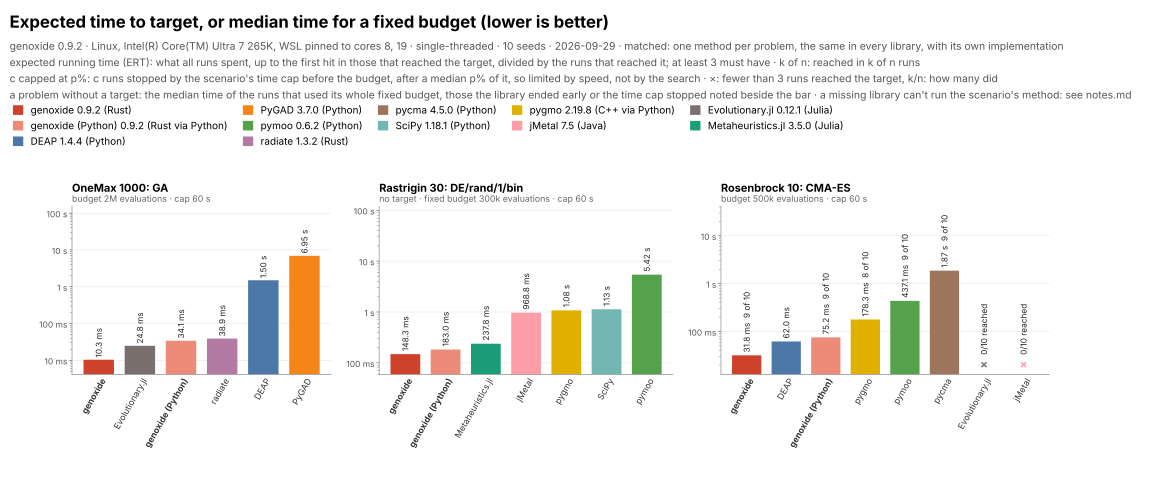
Interactive results, a card per problem: tachsin.gr/projects/genoxide/benchmarks. The methodology, the methods' definitions and a page per library are in docs/benchmarks.

The Rust library

The package covers a subset of the Rust library. These parts are only in Rust:

• SteadyGa and the asynchronous engine, for evaluations of varying duration
• memetic search in Ga, and initial genomes for a population other than trees
• operators of your own
• islands of algorithms other than Ga and De, or of both kinds together
• the stack and column evaluators of gp for values of any type (the package evaluates your own primitives on Python values, a call per node)
• checkpoints in other formats, e.g. JSON through serde
• observers: statistics, a hall of fame and reports
• stop conditions combined with and, and custom ones
• penalty functions for constraints, and the NaN policy: in Python, NaN is always an invalid solution
• advanced settings:
  • CMA-ES: the initial mean
  • PSO: the initial inertia and acceleration (a control can change them during a run), and the maximum velocity
  • DE: population size reduction other than L-SHADE's
  • the rate of UniformCrossover and the weight of ArithmeticCrossover

Some names differ:

Python	Rust
mutation=	.mutate(...)
objective="minimize"	.minimize(), Objective::Minimize
Binary(length), Permutation(length)	Binary::new(len), Permutation::new(len)
BitFlip(rate=...), BitFlip(count=...)	BitFlip::per_gene(rate), BitFlip::count(count), and so for the other mutations
PointCrossover(points)	PointCrossover::k_point(points)
MuPlusLambda(offspring), MuCommaLambda(offspring)	Scheme::MuPlusLambda { lambda }, Scheme::MuCommaLambda { lambda }
Cmaes(restarts="ipop"), Cmaes(restarts="stop")	.restarts(cmaes::Restarts::Ipop), .restarts(cmaes::Restarts::Stop)
Cmaes(covariance="diagonal")	.covariance(cmaes::Covariance::Diagonal)
Pso(ring=k)	.topology(pso::Topology::Ring { neighbors: k })
NelderMead(coefficients="standard"), NelderMead(coefficients=(1.0, 2.0, 0.5, 0.5))	.coefficients(nelder_mead::Coefficients::Standard), .coefficients(nelder_mead::Coefficients::Custom { reflection: 1.0, expansion: 2.0, contraction: 0.5, shrink: 0.5 })
NelderMead(restarts=n)	.restarts(local::Restarts::Random { times: n })
NelderMead(initial_genome=[...])	.initial_genome(Reals::from(vec![...]))
Lbfgsb(gradients="central", difference_step=h)	.gradients(Gradients::Central { step: Some(h) })
Lbfgsb.run(f, gradient=g), gradient=True	Differentiable(|x, gradient| ...)
Mma(method="gcmma")	.method(mma::Method::Gcmma)
Bo(acquisition=gx.UpperConfidenceBound(beta)), Bo(output="log"), Bo(noise=gx.model.gp.Learned(1e-6))	.acquisition(bo::Acquisition::UpperConfidenceBound { beta }), .output(bo::Output::Log), .noise(model::gp::Noise::Learned { min: 1e-6 })
Bo(batch=4, fantasy="liar-min"), bo.run(f, constraints=2)	.batch(4).fantasy(bo::Fantasy::ConstantLiar(bo::Lie::Min)), Constrained::new(2, f)
gx.model.gp.GaussianProcess.fit(genome, points, values), model.predict(points)	GaussianProcess::builder(real).fit(&points, &values)?, model.predict(&x)
Mma.run(f, gradient=True, constraints=m), f returning (value, gradient, g, jacobian)	Constrained::differentiable(m, |x, gradient, g, jacobian| value)
Continuation(method, stages=n, on_stage=f, generations=g, keep="point"), result.stages	Continuation::builder(method).stages(n).on_stage(|stage, _| ...).generations(g).keep(Keep::Point), continuation.stages()
FirstOrder(step="adam", learning_rate=a), FirstOrder(step="nesterov", learning_rate=a, momentum=m), FirstOrder(step="adamw", learning_rate=a, weight_decay=w)	.step(first_order::Step::adam(a)), .step(first_order::Step::nesterov(a, m)), .step(first_order::Step::adamw(a, w))
De(l_shade=n)	De::l_shade(real, n)
De(strategy="rand1"), De(strategy={"p": 0.1, "archive": 1.0})	.strategy(de::Strategy::Rand1), .strategy(de::Strategy::CurrentToPBest { p: 0.1, archive: 1.0 }), and {"max_p", "archive"} for CurrentToPBestRandomP
De(control={"f": 0.5, "cr": 0.9})	.control(de::Control::Fixed { f: 0.5, cr: 0.9 }); {"min_f", "max_f", "cr"} for Dither, {"c"} for Jade, {"memory"} for Shade
De(restarts="never"), De(restarts={"tolerance": 1e-12, "patience": 200})	.restarts(de::Restarts::Never), .restarts(de::Restarts::OnStagnation { tolerance: 1e-12, patience: 200 })
Pbi(theta)	Decomposition::Pbi { theta }
Moead(crossover=gx.DifferentialEvolutionCrossover(f, cr, repair="random"))	.crossover(DifferentialEvolutionCrossover::new(f, cr)?.with_repair(moead::Repair::Random))
gx.gp.Gp(primitives, init=gx.gp.Full((2, 6)))	Gp::builder(set).init(Init::Full { depths: 2..=6 }).build()?
gx.gp.PointMutation(rate=...), gx.gp.ConstantMutation(sigma)	PointMutation::per_node(rate), ConstantMutation::gaussian(sigma)
gx.gp.Mutations([(0.5, gx.gp.SubtreeMutation()), (0.5, gx.gp.HoistMutation())])	Mutations::builder().subtree(0.5).hoist(0.5).build()?
gx.gp.regression.primitives(["add", "mul"], ["x"])	regression::primitives([Math::Add, Math::Mul], ["x"], None)?
gx.gp.regression.Sample(x, y), a point per row	Sample::new(columns, targets)?, a column per variable
problem.regression(linear_scaling=False)	problem.regression().clone().linear_scaling(false)
gx.gp.WithSize(regression)	|tree| Some([regression.evaluate(tree)?, tree.len() as f64])
gx.gp.boolean.Multiplexer(3)	boolean::Multiplexer::new(3)?
Es(recombination="dominant", rho=2, selection="plus", step_sizes="one")	.recombination(es::Recombination::Dominant { rho: 2 }), .selection(es::Selection::Plus), .step_sizes(es::StepSizes::One)
AdaptiveReal(real, initial_step)	AdaptiveReal::new(real, initial_step)?
SelfAdaptiveMutation(learning_rate=tau, min_step=m)	SelfAdaptiveMutation::with_learning_rate(tau)?.with_min_step(m)?
Islands([...], topology="fully_connected")	Islands::builder(vec![...]).topology(Topology::FullyConnected)
islands.islands[i].mutation = ... in a control	islands.islands_mut()[i].mutate_mut()
run(checkpoint=path, checkpoint_every=n)	.checkpoint_every(n, |a| checkpoint::save_file(a, &path)), which saves the algorithm alone; Python's checkpoint holds the settings with it
run(resume=path)	checkpoint::load_file(&path)?, with the algorithm's type
run(control=...), ga.mutation = ... in it	Engine::control(...), *ga.mutate_mut() = ...
ga.mutation_rate = p, de.control = {...}, pso.inertia = w in a control	ga.set_mutation_rate(p)?, de.set_control(...)?, pso.set_inertia(w)?
run(generations=..., time=..., ...)	Stop::generations(...).or(Stop::time(...))
time (seconds)	Stop::time(Duration)
result.seconds	Outcome::elapsed()